As engineers and scientists, we're trying to make the world a better place. In addition to our day jobs, there are things we can do off-hours too. If you can take two hours a week from whatever else you are doing and instead continue to be an engineer, I have a suggestion for you. Please be a mentor. You can be the inspiration to an entire classroom of elementary school students to become engineers and scientists when they grow up. In addition, you get a chance to be a kid and even play with toys - engineering toys.
One way is to be a mentor for a
FIRST Lego League (FLL) team. Every fall, teams of 4-10 elementary and middle school students get a big box of LEGO pieces and a
challenge. By December, they need to have built a fully autonomous robot that will complete as many challenges as possible as well as a presentation on the challenge topic. This year, over 2000 teams participated in regional, national, and international competitions culminating in the
FIRST World Festival in Atlanta, Georgia. It's fun to watch how the kids grow through their participation. The shy learn to speak up, the dominant learn to share, and they all get to experience some fun that they may not normally get in their school day.

(image taken from usfirst.org website - yes, the trophy is made of LEGO pieces)
If you want to work with high-schoolers, FIRST also has two other competitions:
FIRST Tech Challenge and
FIRST Robotics Competition. While the FLL robots are small and plastic, the FTC and FRC robots get heavier and more powerful. FTC robots are around 24" cubes that weigh 5 pounds and the FRC robots get up to 120 pounds and the size of a refrigerator.

(image from usfirst.org website)
40% of FRC participants end up going to engineering school in college. At the FRC finals in Atlanta, I saw 20 colleges with information booths. Athletes aren't the only way to get scholarships now - some schools are giving them out to FRC participants.
Inspire an engineer - get involved. You won't regret it.
The Power.org organization just met in Austin and one of their conversations was on multi-core programming. Some days, I just feel sorry for programmers stuck in the traditional embedded world. This is from an EE-times article:
"The inability of C/C++ code to parallelize coupled with its ubiquity throughout the embedded market is a major issue for multi-core going forward," Heikkila wrote in a follow up email to EE Times. "Any alternative parallel programming languages certainly won't materialize in the embedded market, but instead will more likely gain momentum in a more mainstream computing market before making its way into embedded applications," he added.
And more bad news for current developers
So far, engineers are giving embedded software a low grade of just 2.06 out of five in terms of its readiness for multi-core.
One day, they'll use LabVIEW....
A while ago, I wrote an article about writing parallel programs. The next question is: how do you optimize them?
Note: if you are writing multi-core programs and are coming to NIWeek, please email me (email address on the right). I'd like to talk to you about this topic further. But I digress...
Typically, when optimizing an application, you are trying to make it faster. "Faster" usually means "reduce the time the user observes the task to take". We sometimes call that "wall clock time". Occasionally, there is no outside observer. Instead, you want your task to be less of a disruption on other applications. In that case, you are purely concerned with how much of the resources of the computer, typically the CPU, are being consumed. This consumption could be called "CPU time".
When optimizing for wall clock time, you quickly run into some difficulties.
1) Most profilers give you time of operation in CPU time. A function that goes to sleep for 10 minutes has a CPU time of nearly nothing but a wall clock time of 10 minutes.
For example, if you run this VI with the LabVIEW profiler enabled, it will show that it uses a whopping 46.9 milliseconds
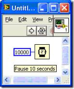
So, you think. Wow, my application took 10 seconds and this function only took 47 milliseconds, I guess my slowdown is elsewhere. And, of course, you would be wrong. Now, this example is pretty silly. No one just adds a sleep for the heck of it. Normally, you'll find "sleep time" in a couple of different places
- Pausing because you need to synchronize with other event. Maybe you go to sleep for 1 second until some external piece of hardware has responded.
- Calls into the OS. Reading from disk and writing from disk occurs in the OS. The CPU time returned by the profiler doesn't normally show time spent in the OS, even though it is consuming CPU cycles.
- Calls into a driver. Some driver calls do their work inside the OS so they are a case of #2. Or, sometimes they get implemented as a LabVIEW sleep, and so they also don't get counted.
- Task swaps. The OS might decide to give some other application some time. This hurts the wall clock time of your application but your profiler won't tell you.
If you want wall to measure wall clock time, you should instead get the tick count of the machine before and after the operation occurs. A tick count uses wall clock time to give you the results. My profiling article shows you how to get the tick count to profile an operation.
2) Things get a bit weirder when you want to try and optimize on a multi-core computer. On a single core machine, you can make your program run faster by either reducing wait time like you saw in #1 or by reducing the CPU time. On a multi core machine, a task can have a shorter wall clock time even though the CPU time and wait time are the same. If you split the CPU work (i.e. CPU time) evenly across two processors, your wall clock time goes down by a factor of 2 but your CPU time is the same.
You can observe this with the Windows task manager. If you have two cores, the task manager will show two graphs of CPU utilization, one for each CPU. You can also use the windows application "perfmon" which gives you a bit more flexible way to observe this.
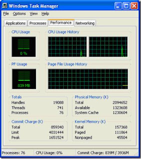
(the CPU Usage History shows 2 graphs, one for each processor)
So, to optimize your application, the trick is to max out both processors. In effect, you are trying to INCREASE the CPU time for the second processor by shifting the processing from CPU 1 to CPU2. It's odd to think of optimizing as increasing processor time, but that's what you are doing.
The problem with using this approach is that increasing the CPU time on the second processor doesn't necessarily reduce wall clock time. Your efforts to make your application more parallel might add CPU work, such as forcing memory copies, that negate the benefit of parallelism.
As an example, the old LabVIEW queue primitives used to copy data into and out of the queues. If you put a big array in a queue, it would spend a lot of time copying the array into the queue and then a lot of time copying it out. To make my application more parallel, I split it into loops and used queues to pass the data between the loops. My CPU utilization was great, 100% on both cores, but my wall clock time was slower because it spent a long time simply copying data around. Fortunately, we learned from that experience and the primitives don't make copies of arrays & clusters any more.
Unfortunately, there's not a really good way to look at this effect right now. Use tick counts to measure your wall clock time and use the profiler to establish a baseline. Then, as you are making changes, make sure the wall clock time is going down and the CPU time is remaining at least constant or only going up slightly.
Labels: LabVIEW, MultiCore, ParallelProgramming, Profiling
If you ever wanted to know how a military radar transmission works, there's a pretty good overview that you can find in this Tektronix Application Note on pages 2-6 It talks about what a radar pulse looks like and why you might modulate the pulse in order to get better performance.
They skipped the most basic type of radar system but Mattel has utilized it to make a really neat and cheap radar gun.
You can use RADAR (technically it's an acronym so it should be capitalized) to tell a number of things about object it's aimed at. The Mattel radar gun gives you the most basic information, speed. It transmits a microwave signal and observes the reflections (if any) that come back from the object. If the object is moving toward or away from the gun, the reflected signal will have a Doppler shift. The amount of frequency shift is proportional to the speed.
Now if you remember your music theory, when you mix two waves of slightly different frequencies together, you get a signal with both frequencies as well as a "beat". The frequency of the beat is the frequency difference between the signals.
Taking advantage of this, the Mattel gun combines the signal it sends and the signal it receives to get the resultant signal, filters out the microwave signals and is left with the beat signal. Get the frequency of the beat signal and it's some simple math to get the velocity of the object.
All this for $30 retail.
Now, notice that the gun doesn't give you position. Radar systems figure out how far the target is away by measuring how long it takes for the signal to reach the target and come back. To do this, they send a pulse and wait for the return and then time the return. The Mattel gun sends a continuous signal rather than a pulse so it has no way of measuring time of flight. That processing would probably also cost a bit more to implement.
Why did I even bother to read this article? Well, I'm seeing some of our customers testing radar systems by simulating return pulses with hardware such as the R-series plug in boards or our Vector Signal Generators and wanted to know a little more about what they were really doing.
Labels: SoftwareDefinedRadio
A device such as a digital oscilloscope uses a high speed a/d converter to acquire the desired signal for some very short duration of time at a very high sampling rate, this acquired data is then transferred through a signal processing engine that may perform some sort of analysis on the data at that point such as an RMS calculation, and then the data is transferred to the main display engine for more math (such as calculating a cursor value) and finally displayed on the screen. So the flow is simple, acquire the data, analyze it to make the measurement, and present the result to the user. For 20 years, NI has used the phrase "acquire, analyze, present" to describe virtual instrumentation. A virtual instrumentation system allowed you to create that oscilloscope yourself out of a PC, a digitizer, and LabVIEW and allowed you to write your own measurement.
However, the phrase "acquire, analyze, present" may misleadingly imply that the phases are discrete when in fact they can be continuous. Why might this be continuous? One example is the processing to perform a trigger. If a scope is going to trigger when the signal exceeds a voltage level, acquisition and analysis must run continuously to digitize the signal and perform some very simple math (comparison) to look for the threshold to be met.
As with all engineering problems, the devil is taking the simple concept and applying it to a need that our customers have. Creating that trigger is subject to two fundamental limitations: the speed at which the trigger criteria can be evaluated and the rate at which the data can be sent from the a/d unit to the trigger computation circuitry. Triggering is typically a hardware operation because it needs to run at a megasample or gigasample rate and it is performed "close" to the a/d converter to handle the data rate of hundreds of megabytes or multiple gigabytes per second being generated.
The march of technology provides some interesting opportunities on the horizon that have been alluded to in past posts. The architecture of a software defined radio (SDR) and an oscilloscope are not that different. The FPGA technology and wideband A/D technology driving SDR is beneficial in T&M applications. The biggest difference is the audience. Whereas the SDR design team consists of C and VHDL programmers working for 12 months on a highly specified design in a high process development environment, the T&M system design team is a few people who know LabVIEW trying to keep up with the changing specs being thrown over the wall and trying to avoid the end product being late even when the design team is late.
The next generation of test equipment will be leveraging the technological power available in the SDR architecture but the ease of use you expect from a T&M instrument to get those difficult measurements made. Imagine the possibilities:
- Write your own math computation for that trigger, compile it, and have it run at the full rate of the hardware.
- Perform calculations on the data at full speed. Need a hundred kilohertz RMS calculation to decode a LVDT? You've got it. Filter or demodulate a 20 MHz communication signal? No problem.
- Take that test that you wrote but have part of it run on an FPGA to speed it up. When that's not good enough, take the whole thing and move it down to the FPGA.
All of these tasks are possible today but some aren't as easy as they could be. The technology is there to accomplish the task, the trick is to expose that power to you. NIWeek is coming up in just over two weeks. I look forward to discussing the possibilities with you there.
Labels: hardware in the loop, Hardware Test, LabVIEW, SoftwareDefinedRadio
In breathless language, the University of Maryland announced
"New Era of "Desktop Supercomputing" Made Possible
with Parallel Processing Power on a Single Chip". If you read the article, you will find no hint of substance whatsoever about why this is so revolutionary and that's a shame because they might actually have something.
The
presentation they made at the Symposium on Parallelism in Algorithms and Architectures is similarly light on detail except for one term I was unfamiliar with so I googled it, a
"PRAM Machine". This machine appears to be a simple (but ill-documented) concept
(From Wellesley CS331 Notes)
A PRAM uses p identical processors ... and [is] able to perform the usual computation of [a typical processor] that is equipped
with a finite amount of local memory. The processors communicate through some shared global memory to which all are connected. The shared memory contains a finite number of memory cells. There is a global clock that sets the pace of the machine executon. In one time-unit period each processor can perform, if so wishes, any or all of the following three
steps:
1. Read from a memory location, global or local;
2. Execute a single RAM operation, and
3. Write to a memory location, global or local.
So really, the only difference between it and a multicore Pentium is that there are probably more than 4 CPUs and that all of the CPUs share a global clock. Interesting but I think the better question is - why did they build it?
It looks like there's a whole set of theory that goes into how to extract parallelism out of algorithms and a PRAM execution model
allows the task to be expressed simply.
For example, suppose you wanted to increment the contents of every element of an array by 1. This type of machine would simply have every processor load one element, increment it, and store it back. If you had the same number of processors as array elements, that operation would take place in exactly one time unit. Perfect parallelization. That particular operation is also found in
"SIMD" machines. Again, the importance is not that a PRAM can implement this operation, it's because there have been languages developed that allow all of this business of scheduling all of the instructions across processors to be abstracted from the programmer.
Interestingly, it looks like we could use these same concepts to schedule LabVIEW code without having to change the diagram at all. Hmm.
Labels: LabVIEW, ParallelProgramming, Supercomputing


